Author Archives: diligentdba

When I was on SQLCruise recently – Buck Woody (b|t) made a interesting statement – that in a room of 23 people, there is over a 50% chance that  two or more have the same birthdays. And sure enough, we did end up having more than two people with same birthday. I was tempted to play with this rather famous problem (there is a great introductory wiki post on it here)  using statistics for a while, and got around to it this weekend. Let us test the hypothesis first.

Given a room of 23 random people, what are chances that two or more of them have the same birthday? 

This problem is a little different from the earlier ones, where we actually knew what the probability in each situation was.

What are chances that two people do NOT share the same birthday? Let us exclude leap years for now..chances that two people do not share the same birthday is 364/365, since one person’s birthday is already a given. In a group of 23 people, there are 253 possible pairs (23*22)/2. So the chances of no two people sharing a birthday is 364/365 multiplied 253 times. The chances of two people sharing a birthday, then, per basics of probability, is 1 – this. Doing the math then – first with T-SQL –

DECLARE @x INTEGER, @NUMBEROFPAIRS INTEGER, @probability_notapair numeric(18, 4), @probability_pair numeric(18, 4)
DECLARE @daysinyear numeric(18,4), @daysinyearminus1 numeric(18, 4)
SELECT @x = 23
SELECT @numberofpairs = (@x*(@x-1)/2)
SELECT @daysinyear = 365
SELECT @daysinyearminus1 = @daysinyear - 1

SELECT @probability_notapair = (@daysinyearminus1/@daysinyear)

SELECT 'Probability of a pair having birthdays' ,1-power(@probability_notapair, @NUMBEROFPAIRS)

In R this is very easily calculated using the line

prod(1-(0:22)/365)

To be aware that prod is just a function that multiplies what it is supplied, it is not a special statistical function of any kind. In this case since the math is really easy, that is all we need to calculate the result.

As we can see it is pretty close to what we got with T-SQL.

We can play around with R a little bit and get a nice graph illustrating the same thing.

positiveprob <- numeric(23) #creatingvectortoholdvalues
#loop and fill values in vector
for (n in 1:23) {
 negativeprob <- 1 - (0:(n - 1))/365
 positiveprob[n] <- 1 - prod(negativeprob) }
#draw graph to show probability
plot(positiveprob, main = 'Graph of birthday probabilites for 23 people', xlab = 'Number of people in room', ylab = 'Probability of same birthdays')

As we can see the probability of two or more people sharing a birthday in a room of about 23 is near 50%. Pretty amazing.

There is a ton of very detailed posts on this rather famous problem, this is just a basic intro for those of you learning stats and R.
1 https://www.scientificamerican.com/article/bring-science-home-probability-birthday-paradox/

2 http://blog.revolutionanalytics.com/2012/06/simulating-the-birthday-problem-with-data-derived-probabilities.html

Thanks for reading!!

In the previous post I demonstrated the use of binomial formula to calculate probabilities of events occurring in certain situations. In this post am going to explore the same situation with a bigger sample set. Let us assume, for example, that instead of 7 smokers we had 100 smokers. We want to know what are the chances that a maximum of 35 of them have a serious lung disease. Going by the Binomial formula illustrated in the previous post that would mean a whole lot of calculations – calculating the probability of every situation less than 35 and then stick the values into the formula to derive an answer. That is a very laborious way to derive a result, even if we are using an automated process to do it.  An easier way to do it is to use the normal distribution, or central limit theorem. My post on the theorem illustrates that a sample will follow normal distribution if the sample size is large enough. We will use that as well as the rules around determining probabilities in a normal distribution, to arrive at the probability in this case.
Problem: I have a group of 100 friends who are smokers.  The probability of a random smoker having lung disease is 0.3. What are chances that a maximum of 35 people wind up with lung disease?

Step 1: How do I know my problem fits this particular statistical solution?
To determine whether n is large enough to use what statisticians call the normal approximation to the binomial, both of the following conditions must hold:

In this case 100*0.3 = 30, which is way greater than 10. The second condition 100*0.7 is also 70 and way greater than 10. So we are good to proceed.

2 Statistically stated, we need to find P(x<=35)

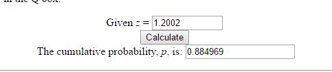
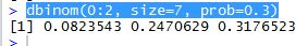
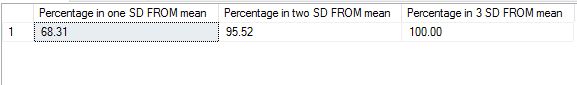
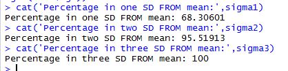
3 The formula to use now is  where ‘meu’ in the numerator is the mean and sigma, the denominator is the standard deviation. Let us use some tried and trusted t-sql to arrive at this value.

4 We use 35 as x, but we add 0.5 as suggested ‘corrective value’ to it. Running T-SQL to get z value as below:

DECLARE @X numeric(10,4), @p numeric(10, 4), @n numeric
(10, 4), @Z NUMERIC(10, 4)
DECLARE @MEAN NUMERIC(10, 4), @VARIANCE NUMERIC(10, 4), @SD NUMERIC(10, 4)
SELECT @X = 35.5
SELECT @P = 0.3
SELECT @N = 100
SELECT @MEAN = @N*@p
SELECT @VARIANCE = @N*@p*(1-@p)
SELECT @SD = SQRT(@VARIANCE)
SELECT @Z = (@X-@MEAN)/@SD
SELECT @Z as 'Z value'

5 To calculate probability from Z value, we can use Z value tables. There are also plenty of online calculators available – I used this one.  I get probability to be 0.884969.

6 The same calculation can be achieved with great ease in R by just saying

pbinom(35,size=100,prob=0.3)

The result I get is very close to above.

You can get the same result by calling the R function from within TSQL as below

EXEC sp_execute_external_script
 @language = N'R'
 ,@script = N'x<-pbinom(35,size=100,prob=0.3);
 print(x);'
 ,@input_data_1 = N'SELECT 1;'

In other words, there is a 88.39 percent chance that 35 out of 100 smokers end up with lung disease. Thank you for reading!

In a previous post I explained the basics of probability. In this post I will use some of those principles to see how to solve certain problems. I will pick a very simple problem that I found in a statistics textbook. Suppose I have 7 friends who are smokers. The probability that a random smoker will develop a lung condition is 0.3. What is the probability that a maximum of 2 of them will develop a severe lung condition? To apply the binomial formula for this problem – I need the following conditions to be met:

1 The trials are independent
2 The number of trials, n is fixed.
3 Each trial outcome can be a success or a failure
4 The probability of success in each case is the same.

Applying these rules –
1 The 7 smoking friends are not related or from the same group. (This is important as one friend’s habits can influence another and that does not make for an independent trial).
2 They smoke approximately at the same rate.
3 Either they get a lung disease or they don’t. We are not considering other issues they may have because of smoking.
4 Since all these conditions are met, the probability of each of them getting a lung disease is more or less the same.

The binomial formula given that
x = total number of “successes” (pass or fail, heads or tails etc.)
P = probability of a success on an individual trial
n = number of trials
q= 1 – p – is as below:

For those not math savvy the ! stands for factorial of a number. In above example n equals 7. x, The number of ‘successes’ (morbid, i know, to define a lung condition as a success but just an example) we are looking for is 2. p is given to be 0. and q is 1 – 0.3 which is 0.7.  Now, given the rules of probability – we need to add probability of 0 or none having a lung condition, 1 person having a lung condition and 2 having a lung condition – to see what is the probability of a maximum of 2 having a lung condition. Let us look at doing this with T-SQL first, then with R and then calling the R script from within T-SQL.

1 Using T-SQL:

There are a lot of different ways to write the simple code of calculating factorial. I found this one to be most handy and reused it. I created the user defined function as ‘factorial’ and used the same code below to calculate probabilities of 0.1 or 2 people getting a lung illness. If we add the 3 together we get the total probability of the maximum of 2 people getting a lung illness – which is about 0.65 or 65 %.

DECLARE @n decimal(10,2), @x decimal(10, 2), @p decimal(10, 2), @q decimal(10, 2)
DECLARE @p0 decimal(10, 2), @p1 decimal(10, 2), @p2 decimal(10, 2), @n1 decimal(10, 2), @n2 decimal(10, 2), @n3 decimal(10, 2)
SELECT @n = 7, @x = 0, @p = 0.3,@q=0.7
SELECT @x = 0
SELECT @n1 = dbo.factorial(@n) 
SELECT @n2 = dbo.factorial(@n-@x)
SELECT @n3 = 1

SELECT @p1 = ( @n1/(@n2 * @n3))*power(@p, @x)*power(@q,@n-@x)
select @p1 as 'Probability of 0 people getting lung illness'

SELECT @x = 1
SELECT @p1 = ( @n/@x)*power(@p, @x)*power(@q,@n-@x)
select @p1 as 'Probability of 1 person getting lung illness'

SELECT @x = 2
SELECT @n1 = dbo.factorial(@n) 
SELECT @n2 = dbo.factorial(@n-@x)
SELECT @n3 = dbo.factorial(@x)
SELECT @p2 = ( @n1/(@n2 * @n3))*power(@p, @x)*power(@q,@n-@x)
select @p2 as 'Probability of 2 people getting lung illness'

Results are as below:

2 Using R:

The R function for this is seriously simple, one line call as below.

dbinom(0:2, size=7, prob=0.3)

My results, almost exactly the same as what we got with T-SQL.

3 Calling R from T-SQL:

Instead of writing all that code i can simply call this function from with TSQL –

EXEC sp_execute_external_script
 @language = N'R'
 ,@script = N'x<-dbinom(0:2, size=7, prob=0.3);
 print(x);'
 ,@input_data_1 = N'SELECT 1;'

Results as below:

It is a LOT of fun to get our numbers to tie in more than one way. Thanks for reading.

In this post am going to introduce into some of the basic principles of probability – and use it in other posts going forward. Quite a number of people would have learned these things in high school math and then forgotten – I personally needed a refresher. These concepts are very useful if we can keep them fresh in mind while dealing with more advanced programming in R and data analysis.
Probability is an important statistical and mathematical concept to understand. In simple terms – probability refers to the chances of possible outcome of an event occurring within the domain of multiple outcomes. Probability is indicated by a whole number – with 0 meaning that the outcome has no chance of occurring and 1 meaning that the outcome is certain to happen. So it is mathematically represented as P(event) = (# of outcomes in event / total # of outcomes). In addition to understanding this simple thing, we will also look at a basic example of conditional probability and independent events.

Let us take an example to study this more in detail.
I am going to use the same  dataset that I used for normal distribution – life expectancy from WHO. My dataset has 5 fields – Country, Year, Gender, Age. Am going to answer some basic questions on probability with this dataset.

1 What is the probability that a random person selected is female?  It is the total # of female persons divided by all persons, which gives us 0.6. (am not putting out the code as this is just very basic stuff). Conversely, the ‘complement rule’ as it is called means the probabilty of someone being male is 0.4. This can be computed as 1 – 0.6 or total # of men /total in sample. Since being both male and female is not possible, these two events can be considered mutually exclusive.

2 Let us look at some conditional probability. What is the probability that a female is selected given that you only have people over 50? The formula for this is probability of selecting a female over 50 divided by probability of selecting someone over 50.

DECLARE @COUNT NUMERIC(8, 2), @COUNTFEMALE NUMERIC(8, 2),@COUNTMALE NUMERIC(8, 2)
SELECT @COUNTFEMALE = COUNT(*) FROM [dbo].[WHO_LifeExpectancy] WHERE GENDER = 'female' and AGE > 50
SELECT @COUNT = COUNT(*) FROM [dbo].[WHO_LifeExpectancy]
SELECT 'PROBABILITY OF A FEMALE OVER 80' , @COUNTFEMALE/@COUNT
SELECT @COUNTMALE = COUNT(*) FROM [dbo].[WHO_LifeExpectancy] WHERE age > 50
SELECT @COUNT = COUNT(*) FROM [dbo].[WHO_LifeExpectancy]
SELECT 'PROBABILITY OF ANY RANDOM PERSON over 50' , @COUNTMALE/@COUNT
SELECT 'PROBABILITY OF SELECTING A FEMALE FROM OVER 50', @COUNTFEMALE/@COUNTMALE

3 Do we know if these two events are dependent or independent of each other? That is , is does selecting a female over 50 affect the probability of selecting any person over 50? To find this out we have to apply the formula for independence – which is that the probability of their intersection should equal the product of their unconditional probabilities..that is probability of female over 50 multiplied by probability of female should equal probability of female and 50.

DECLARE @pro50andfemale numeric(12, 2), @total numeric(12, 2), @female numeric(12, 2), @fifty numeric(12, 2)
select @pro50andfemale= count(*) from [dbo].[WHO_LifeExpectancy] where age > 50 and gender = 'female'
select @total = count(*) from [dbo].[WHO_LifeExpectancy]
select 'Probability of 50 and female' ,round(@pro50andfemale/@total, 2)

select @female = count(*) from [dbo].[WHO_LifeExpectancy] where gender = 'female'
select 'Probability of female', @female/@total
select @fifty = count(*) from [dbo].[WHO_LifeExpectancy] where age > 50
select 'Probability of fifty', @fifty/@total
select 'Are these independent ', round((@female/@total), 2)*round((@fifty/@total), 2)

Results are as below..as we can see, the highlighted probability #s are very close suggesting that these two events are largely independent.

From the next post am going to look into some of these concepts with R and do some real data analysis with them. Thanks for reading.

This week’s blog post is rather simple. One of the main characteristics of a data set involving classes, or discrete variables – are frequencies. The number of times each data element or class is observed is called its frequency. A table that displays the discrete variable and number of times it occurs in the data set is called a ‘Frequency Table’.A frequency table usually has frequency, percent or relative frequency expressed in % (the percentage of occurrences), cumulative frequency – the number of times all the preceding values have occurred and Cumulative Relative Frequency which is the ratio of cumulative frequency to size of sample (this can also be expressed as a percent if so desired).

For creating this I used the same data set I used for studying Simpson’s Paradox
To remember that variables we are deriving frequency for should be DISCRETE  in nature and each instance of the variable should be related/comparable to another in some way. If we are interested in cumulative values – those should make some kind of sense..so just summing all records before a name, or before a product(even though those classify as discrete), may not really make sense in most situations .In this case my variable is the age cohort, so summing whatever is below a certain age cohort can be useful data.

My TSQL for this is as below:

DECLARE @totalcount numeric(18, 2)
SELECT @totalcount = COUNT(*) FROM [dbo].[paradox_data]
;WITH agecte AS 
(
 SELECT [agecohort], c = COUNT(agecohort) 
 FROM [dbo].[paradox_data]
 GROUP BY [AgeCohort] 
)
SELECT agecte.[agecohort], c as frequency,(agecte.c/@totalcount)*100 AS [percent], 
 cumulativefrequency = SUM(c) OVER (ORDER BY [agecohort] ROWS UNBOUNDED PRECEDING),
 cumulativepercent = ((SUM(c) OVER (ORDER BY [agecohort] ROWS UNBOUNDED PRECEDING))/@totalcount)*100
FROM agecte
ORDER BY agecte.[agecohort];

My results are as below. I have 1000 records in the table. This tells me that I have 82 occurences of age cohort 0-5, 8.2% of my dataset is from this bracket, 82 again is the cumulative frequency since this is the first record and 8.2 cumulative percent. For the next bracket 06-12 I have 175 occurences, 17.5 %, 257 occurences of age below 12, and 25.7 % of my data is in this age bracket. And so on.

Let us try the same thing with R. As it is with most R code, part of this is already written in a neat little function here. I did however, find some issues with this code and had to modify it. The main issue was that the function was calculating ‘length’ of the dataframe (in sql terms – number of records) from the variable – and R kept returning a value of ‘1’. The correct way to calculate number of records is to specify the field name after the dataframe, so when I did that it was able to get to the total number of records. This is a little nuance/trick with R that gets many sql people confused, and was happy to have figured it out. I do not know of a ‘macro’ or a generalised function that can pull this value so I had to stick it to the function. It will be different if you use another field for sure. The modified function and value it returns is as below.

##This is my code to initiate R and bring in the dataset

install.packages("RODBC")
library(RODBC)

cn <- odbcDriverConnect(connection="Driver={SQL Server Native Client 11.0};server=MALATH-PC\\SQL01;database=paradox_data;Uid=sa;Pwd=mypwd")data <- sqlQuery(cn, 'select agecohort from [dbo].[paradox_data]')

make_freq_table <- function( lcl_list )


 {
 ## This function will create a frequency table for 
 ## the one variable sent to it where that 
 ## table gives the items, the frequency, the relative 
 ## frequeny, the cumulative frequency, the relative
 ## cumulative frequency
 ## The actual result of this function is a data frame 
 ## holding that table.
 lcl_freq <- table( lcl_list )
 

##had to change this from original code to pull correct length.

lcl_size <- length( lcl_list$agecohort )
 lcl_df <- data.frame( lcl_freq )
 names( lcl_df ) <- c("Items","Freq")
 lcl_values <- as.numeric( lcl_freq )
 lcl_df$rel_freq_percent <- (lcl_values / lcl_size)*100
 lcl_df$cumul_freq <- cumsum( lcl_values )
 lcl_df$rel_cumul_freq_percent <- (cumsum( lcl_values ) / lcl_size)*100
lcl_df
 } 

make_freq_table(data) 

The result I get is as below and is the same as what I got with T-SQL.

Since this is a rather simple example that is 100 percent do-able in TSQL – I did not find the need to do it by calling R from within it. It did help me learn some nuances about R though.

Thanks for reading.

I am resuming technical blogging after a gap of nearly a month. I will continue to blog my re learning of statistics and basic concepts, and illustrate them to the best of my ability using R and T-SQL where appropriate.

For this week I have chosen a statistical concept called ‘Empirical Rule’.

The empirical rule is a test to determine if or not the dataset belongs to a normal distribution.

• 68% of data falls within the first standard deviation from the mean.
• 95% fall within two standard deviations.
• 99.7% fall within three standard deviations.

The rule is also called the 68-95-99 7 Rule or the Three Sigma Rule. The basic reason to test if a dataset follows this rule is to determine whether or not it is a normal distribution. When it is normally distributed and follows the bell curve – it lends itself easily to a variety of statistical analysis, especially forecasting. There are many other tests for normalisation that are more rigorous than this – and the wiki link has a good summary of those, but this is a basic and easy test.
For my test purpose I used the free dataset from WHO 0n life expectancies around the globe. It can be found here. I imported this dataset into sql server. I ran a simple TSQL script to find out if this dataset satisfies the empirical rule.

DECLARE @sdev numeric(18,2), @mean numeric(18, 2), @sigma1 numeric(18, 2), @sigma2 numeric(18, 2), @sigma3 numeric(18, 2)
DECLARE @totalcount numeric(18, 2)
SELECT @sdev = SQRT(var(age)) FROM [dbo].[WHO_LifeExpectancy]
SELECT @mean = sum(age)/count(*) FROM [dbo].[WHO_LifeExpectancy]
SELECT @totalcount = count(*) FROM [dbo].[WHO_LifeExpectancy]
SELECT @sigma1 = (count(*)/@totalcount)*100 FROM [dbo].[WHO_LifeExpectancy] WHERE age >= @mean-@sdev and age<= @mean+@sdev
SELECT @sigma2 = (count(*)/@totalcount)*100 FROM [dbo].[WHO_LifeExpectancy] WHERE age >= @mean-(2*@sdev) and age<= @mean+(2*@sdev)
SELECT @sigma3 = (count(*)/@totalcount)*100 FROM [dbo].[WHO_LifeExpectancy] WHERE age >= @mean-(3*@sdev) and age<= @mean+(3*@sdev)

SELECT @sigma1 AS 'Percentage in one SD FROM mean', @sigma2 AS 'Percentage in two SD FROM mean', 
@sigma3 as 'Percentage in 3 SD FROM mean'

The results I got are as below. As we can see ,68.31 % of data falls between one difference of mean and standard deviation, 95 % falls between two differences and 100% falls between 3. This is a near perfect normal distribution – one that lends itself to statistical analysis very easily.

To do the same analysis in R, I used script as below:

install.packages("RODBC")
library(RODBC)

cn <- odbcDriverConnect(connection="Driver={SQL Server Native Client 11.0};server=MALATH-PC\\SQL01;database=WorldHealth;Uid=sa;Pwd=Mysql1")
data <- sqlQuery(cn, 'select age from [dbo].[WHO_LifeExpectancy] where age is not null')
agemean<-mean(data$age)
agesd<-sd(data$age)
sigma1<-(sum(data$age>=agemean-agesd & data$age<=agemean+agesd)/length(data$age))*100
sigma2<-(sum(data$age>=agemean-(2*agesd) & data$age<=agemean+(2*agesd))/length(data$age))*100
sigma3<-(sum(data$age>=agemean-(3*agesd) & data$age<=agemean+(3*agesd))/length(data$age))*100
cat('Percentage in one SD FROM mean:',sigma1)
cat('Percentage in two SD FROM mean:',sigma2)
cat('Percentage in three SD FROM mean:',sigma3)

My results are as below:

I can use the same script within TSQL and call it –

EXEC sp_execute_external_script
 @language = N'R'
 ,@script = N'agemean<-mean(InputDataSet$age)
agesd<-sd(InputDataSet$age)
sigma1<-(sum(InputDataSet$age>=agemean-agesd & InputDataSet$age<=agemean+agesd)/length(InputDataSet$age))*100
sigma2<-(sum(InputDataSet$age>=agemean-(2*agesd) & InputDataSet$age<=agemean+(2*agesd))/length(InputDataSet$age))*100
sigma3<-(sum(InputDataSet$age>=agemean-(3*agesd) & InputDataSet$age<=agemean+(3*agesd))/length(InputDataSet$age))*100
print(sigma1)
print(sigma2)
print(sigma3)'
 ,@input_data_1 = N'select age from [dbo].[WHO_LifeExpectancy] where age is not null;'

As we can see, the results are exactly the same in all 3 methods. We can also draw a bell curve with this data in R and see that it is a perfect curve, proving that the data is from a normally distributed set. The code I wrote to draw the graph is as below:

lower_bound <- agemean - agesd * 3
upper_bound <- agemean + agesd * 3
x <- seq(-3, 3, length = 1000) * agesd + agemean
y <- dnorm(x, agemean, agesd)
plot(x, y, type="n", xlab = "Life Expectancy", ylab = "", main = "Distribution of Life Expectancies", axes = FALSE)
lines(x, y)
sd_axis_bounds = 5
axis_bounds <- seq(-sd_axis_bounds * agesd + agemean, sd_axis_bounds * agesd + agemean, by = agesd)
axis(side = 1, at = axis_bounds, pos = 0)