How I used AI for this post
ChatGPT to generate images based on info specifically provided by me,including examples.
Grammarly to catch grammar and sentence construction errors.
In Part 1, we looked into foundational elements of DiskANN. The example we used was:
“boots for hiking in the rain”.
Vectors are represented as nodes in the DiskANN graph structure, and Edges are connections between those nodes. ‘Vamana’ and ‘RobustPrune’ make that graph sparse without destroying useful routes. At query time, ‘greedy graph traversal’ used a candidate list to find vectors increasingly similar to the query.
Conceptually the search looked like this:
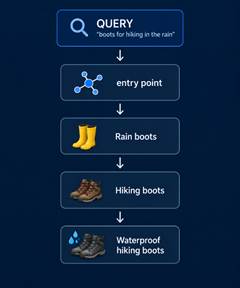
At this point, the consideration becomes – ‘What if the graph and all of its vectors don’t fit in memory?’
If every step of graph traversal had to wait for an arbitrary SSD read, the navigation could become painfully slow.
Why not just put everything in RAM?
Suppose our product embedding has 768 dimensions, with each dimension stored as a 32-bit floating-point number.
One vector requires roughly – 768 dimensions × 4 bytes = 3,072 bytes ≈ 3 KB
When we scale upto a billion of them, we get to 3 KB × 1,000,000,000 ≈ 3 TB
That’s before we even consider accounting for the graph and other index structures. At this scale, “keep the entire index in RAM” becomes an expensive design constraint. SSDs give us vastly more affordable capacity. But SSDs introduce another problem. RAM access is extremely fast. SSD access is much slower, particularly when an algorithm repeatedly asks for small pieces of data from different locations.
Imagine our search moving through the rain-boots graph:
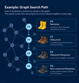
If every expansion means:
visit P4 → wait for SSD
visit P7 → wait for SSD
visit P2 → wait for SSD
visit P9 → wait for SSD
Then storage latency starts controlling search latency.
An efficient search needs to keep enough information in RAM to make good navigation decisions, while touching the SSD only when necessary. That is what makes Product Quantization important to understand.
Product Quantization: a smaller map in memory
One of our product vectors stands for:
“Men’s waterproof hiking boots” and may be represented as
[0.12, -0.73, 0.41, 0.08, …]
The vector holds many floating-point numbers. It is not always essential to employ the full-precision vector when assessing whether a candidate merits further investigation. Product Quantization, or PQ, gives us a cheap approximation.
Before the index is searched, DiskANN trains a PQ model on representative vectors from the dataset. Training generates compact codebooks that compress dataset vectors for efficient search.
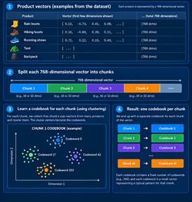
PQ trades precision for memory. The compressed vector is not identical to the original vector. Distances calculated from it are approximate. The goal of ANN Search is to identify promising candidates; not necessarily make the final ranking decision from every candidate it encounters.
For our rain boots query that looks like “boots for hiking in the rain” –
PQ can help us cheaply estimate the approximate distance.
Vectors/Nodes Distance
Waterproof hiking boots 0.12
Rain boots 0.17
Snow boots 0.29
Running shoes 0.61
Camping tent 0.82
That may be enough information to decide where the graph search should go next.
PQ – ‘cheap screening stage.’
Imagine you have one billion shoes to pick from but can only have time to look at 20. You don’t need each pair’s description. You only need the 20 that are worth your time. The summary helps you screen those 20. Then you retrieve the full documents only for the shoes that matter. DiskANN uses compressed representations for the same reason.
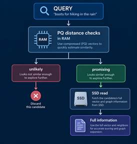
RAM helps answer “where should I look?”
SSD holds the larger information needed when it is needed and when the graph traversal reaches the point where it is needed after the greedy-search iteration.
What lives on SSD?
For a graph node such as:
P17 = Waterproof hiking boots
The vector search cares about two things:
P17, the vector, and its graph neighbors, say
P42 – running boots
P83 – rain boots
P109 – snow boots.
When search decides that P17 is worth expanding, it needs to discover:
“What are the other nodes I can reach from P17?” It then goes to disk to reach the complete set of embeddings for P17 and gets its neighbors.
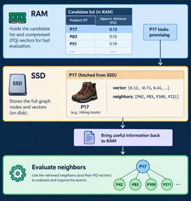
It does not read the whole index from SSD. It does selective reads driven by graph search. But SSD reads are still expensive.
The algorithm has reduced the amount of data kept in RAM. But it is still read intensive, because it still needs to fetch data for each of the neighbors, and each of that adds up to a read. The reads are sequential, which means CPU spends time waiting for storage.
DiskANN is about evaluating a list of candidates, not just one at a time.
It maintains a candidate frontier. That leads to ‘beam search’.
Beam search: give the SSD several things to do
From the candidate list, instead of doing the loop of reading the node we want – wait process-read the next node, we can work several promising candidates simultaneously, as below.
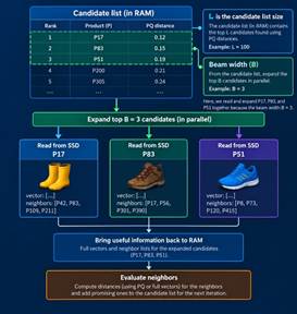
That gives the storage device more parallel work and helps hide some of the latency of individual reads. The SSD-index design notes in the DiskANN repository explicitly call for beam search to explore more than one neighbor at a time and increase SSD queue depth, with asynchronous I/O used to hide waiting time.
This is why beam width becomes much more interesting once DiskANN moves to disk. Beam width depends on more than just the number of expanded candidates.
Beam width facilitates I/O parallelism by enabling simultaneous retrieval of multiple promising graph nodes, rather than performing each SSD access in a sequential manner. It may also be noteworthy that L and beam width are not the same thing.
L determines the permitted breadth of the frontier. Beam width determines the number of candidates expanded at once.
For example, L = 100 beam width = 4 does not mean we are reading 100 nodes from SSD simultaneously. It means keeping up to 100 promising candidates. From amongst them, choose a small batch of 4 to expand and search together.
On an SSD-backed index, the second knob also affects how effectively we can use the storage device. Certain graph nodes exhibit higher popularity compared to others, resulting in more frequent visits. such nodes are cached for further processing. These optimizes reads from SSD even further.
Putting the pieces together
Let’s run our rain boots query again.
“Boots for hiking in the rain”
- The query is vectorized, then graph search starts in RAM.
- PQ-compressed vectors speed up candidate selection, and cached graph nodes improve access efficiency.
- The candidate list (L) holds the best options found so far, while beam width determines how many can be expanded at once.
- Only those promising nodes require selective reading from SSD, where the larger graph and vector data live.
This lets DiskANN search for datasets far larger than RAM without reading the entire index from disk.
PQ helps make large numbers of approximate distance evaluations cheap enough to guide the search.
The graph indicates the permitted destination nodes. Takeaways are as below –
L determines how broad a set of possibilities we keep alive.
The cache prevents us from repeatedly fetching useful nodes from disk.
Beam search enables concurrent SSD operations by expanding multiple promising nodes.
The SSD provides the capacity to hold an index far larger than available RAM.
Exploring only a tiny, useful portion of the vector space while still recovering the true nearest neighbors are often enough to achieve high recall.
Summary of terminologies used so far –
| Term | Simple meaning |
| SSD index | the large graph/vector store that does not need to fit entirely in RAM |
| PQ | a compressed approximation of vectors used to make candidate evaluation cheaper |
| PQ code | the compact representation of a vector |
| Cache | useful graph data we keep in RAM to avoid repeated SSD reads |
| Cache hit | The node we need is already in RAM |
| Cache miss | we have to fetch the node from SSD |
| SSD read | fetching graph/vector information for a node we want to explore |
| L | how broad a candidate frontier we maintain |
| Beam width | how many promising candidates we expand together |
| I/O parallelism | having multiple SSD reads in flight instead of waiting for them one at a time |
| Recall | whether all these shortcuts still find the true nearest neighbors often enough |
In the next and final part, we can look at how to tweak each of these knobs operationally: R, alpha, L, beam width, PQ size, memory budget, recall, latency and actually tune a DiskANN index.
