Referrals have never been more important in the job market. They’re no longer nice to have; in many cases, they’re what gets your résumé through the door.
I’ve been fortunate to land jobs through referrals throughout my career, and I’ve referred many people to positions at organizations where I’ve worked. A recent experience with a friend made me think about some common misunderstandings around referrals—both giving them and receiving them.
A friend of mine, whom I’ll call J, had been out of work for several months. J and their partner were under considerable emotional stress and financial pressure. They had been through a few interviews with no follow ups or offers. One day I got a chat message. Our conversation went as below.
“You won’t believe who referred me for this job!”
“That’s great,” I said. “Do you have an interview?”
“Yes, in two days. I’m feeling really positive about it. I never thought this person would refer me—or that they thought so highly of me.”
“Did they write you a recommendation? Did you see what they said?”
“No. They just told me they referred me, and the interview call came soon after.”
I congratulated J but added one caution: “Go in with enthusiasm, but remember there may be other candidates too.”
J brushed it off. “Of course there are other candidates. But this person thought I was the best, so there you go!”
I left it at that and wished J luck.
Two days later, J called again. They hadn’t gotten the job.
“I think you were trying to warn me,” J said. “That person referred several people, and one of them got the job.”
I told J I was sorry, then explained what I had been trying to say: a referral doesn’t necessarily mean the referrer believes you are the best candidate. Sometimes it does. Sometimes it simply means, “I think this person is worth talking to.”
Then I asked: “Would you have done anything differently if you had known?”
J said yes.
“The person they hired is much more experienced than I am. I’ve seen their work, blogs, and presentations. They have more than a decade of experience on me. If I had known I was competing with people like that, I wouldn’t have gone. The interview was 100 miles away and had to be in person. I spent an entire day on it.”
J’s experience felt familiar because I’ve made similar assumptions myself.
Once, I assumed that someone referring me believed I was the strongest person for the job. Another time, I assumed the other candidates would have roughly the same level of experience and skills that I did. Both assumptions were wrong, and both led to unnecessary disappointment.
In any scenario, we rarely know who else is competing for a position. But a referral can create an additional expectation: ‘Someone put my name forward, so they must think I have an especially good chance’.
That isn’t always what a referral means.
Over time, I’ve developed a few personal guidelines to make referrals clearer and manage expectations on both sides.
When I refer someone
If I can, I refer only one person for a particular position. Usually, it’s someone I know well enough to genuinely vouch for. (A strong community contact, someone I worked with). I find this rule particularly important when the person I am referring is a minority (A woman, a person of color etc). I think this is valuable (to me) because minority folks are most commonly pitted against unfair competition.
That’s my personal approach, not a universal rule. Other people use referrals differently. Some see a referral as a strong endorsement. Others see it simply as a way to help a qualified person get their résumé in front of a hiring manager.
Neither approach is necessarily wrong. The important thing is understanding which kind of referral you’re receiving.
When someone refers me
I ask a couple of questions.
First, I ask whether they’ve referred other candidates for the same position.
Second, I ask what the referral means: ‘Are you specifically recommending me for this role, or are you helping me get an opportunity to interview?’
That distinction matters.
I also try to understand the likely competition. Who already works at the organization? What level of experience does the position appear to require? Is this the kind of opening that will attract a large and highly qualified pool?
None of this guarantees an outcome. But it helps me decide how much time, travel, preparation, and emotional energy I want to invest.
A referral is valuable. It can get you noticed in a crowded market and open a door that might otherwise remain closed.
But an open door is not a job offer.
Perhaps the healthiest way to think about a referral is this: ‘someone believes you deserve a chance to be considered’.
Sometimes it means more than that. But unless you know otherwise, it’s probably best not to assume it does.
How I used AI for this post: For image generation. Grammarly for spell check. Voice is entirely mine.
In Part 1, we saw how ‘Vamana’ represents vectors as nodes, connects them with edges, and uses greedy graph traversal to avoid comparing a query against every vector in the dataset. In Part 2, we investigated how PQ gave us compact representations for inexpensive distance calculations, caching kept useful graph nodes close, how SSDs provided capacity, and beam search allowed multiple promising nodes to be expanded together.
In this last part, we will be exploring how we use the parameters to tune DiskANN.
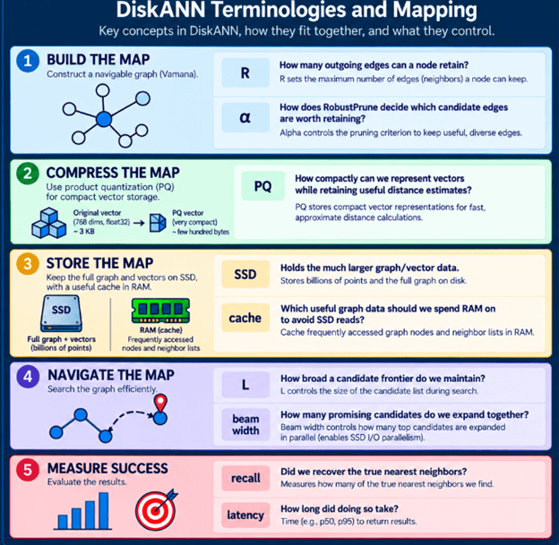
DiskANN offers several settings that control graph construction and search aggressiveness. Those settings trade recall, latency and memory against one another, There is no correct setting that is universal. It is therefore useful to understand what each parameter changes physically inside the algorithm.
Some parameters affect the graph. Others affect how we search that graph.
R and alpha shape the map. L and beam width control how we navigate it.
Changing fundamental build parameters such as R or alpha means changing the graph itself, so evaluating them involves rebuilding the index.
Changing L or beam width can change query behavior without rebuilding the graph.
1.R — maximum roads/edges per node
During graph construction, we may identify multiple candidate neighboring nodes, or edges, associated with a given node. We do not need to retain every edge, so \(R\) sets an upper limit on a node’s outgoing edges—its edge budget.
Larger graphs require more storage, while expanding nodes increases search work. A higher *R* provides richer connectivity and more routes but requires additional index storage and construction time; *R* = 64 does not mean every node has exactly 64 neighbors. It only means pruning allows up to 64 connections per node. Tradeoffs:
More edges create more routes to search in the vector space, but each route adds computational cost. The larger the search, the longer the index is going to take to build and the longer a query is going to take. The sweet spot is finding enough nodes that add value and make results decent quality wise.
2. Alpha — which roads are worth keeping?
R specifies the permitted number of edges. It does not tell us which ones are useful. That is the job of pruning. Suppose node ‘Waterproof hiking boots have two neighbors’ Rain boots’ and ‘Trail shoes.
‘Rain boots’ is close to ‘Waterproof hiking boots. ‘Waterproof hiking boots’ is also close to ‘Trail shoes. But ‘Trail Shoes’ and ‘Rain boots’ are themselves remarkably close. If we already retain ‘Waterproof Rain boots’ -> ‘Rain boots’ then ‘Waterproof Rain boots’ → ‘Trail Shoes’ may add little navigational value because ‘Trail Shoe’’s region can already be reached through A. This is the intuition behind RobustPrune.
Rather than simply selecting the R closest vectors, Vamana uses RobustPrune to determine whether candidate edges provide useful routes or are sufficiently covered by edges already selected. The parameter alpha influences this pruning criterion, changing which edges survive and therefore the topology and navigability of the resulting graph.
Trade-off: Changing alpha can produce a more navigable graph and affect recall, but it also changes graph construction and requires rebuilding the index to retune.
3. L — how hard are we willing to search?
Once constructed, the graph is ready for querying.
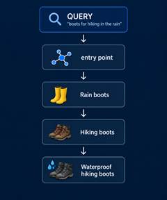
A query arrives:
“Boots for hiking in the rain” It becomes query vector q, and graph traversal begins.
During the search, we maintain promising candidates – such as below:
Parameter L controls the size of this list. A small L means we are willing to keep a narrow search frontier. A smaller L may limit the list to P17, P83 and P 51.
A larger L keeps more possibilities open, including P17, P83, P51, P20, P91, P33, P74, P82, and others. Greedy graph search can mistake the best immediate direction for the best route. A broader frontier gives the algorithm more opportunities to recover from those decisions.
Trade-offs: Larger L improves recall by exploring more of the graph, but requires more distance calculations, node expansions and potentially SSD reads—raising query latency and resource usage.
4.Beam width — the amount of work issued parallelly.
Assume that *L*, the number of candidates being evaluated, is 100. Our candidate list may contain up to roughly that search breadth. That does not mean we have expanded 100 candidates simultaneously. That depends on ‘beam width’. If beam width = 3, then we may only select 3 candidates out of the list of 100 to expand at any given time. L refers to the number of promising possibilities retained, whereas beam width denotes the number of possibilities expanded simultaneously. SSD performance depends on simultaneous expansion to handle multiple outstanding I/O operations.
DiskANN’s SSD design uses beam search and asynchronous I/O to increase the amount of useful work the SSD can have in flight.
Tradeoffs: Increasing beam width exposes more I/O parallelism, helping DiskANN hide SSD latency. Beyond the SSD’s optimal capacity, larger beams cause unnecessary reads, computation, and I/O contention. The sweet spot is enough parallelism to keep the SSD busy—not maximize parallelism.
5.PQ — required RAM precision
Our original vectors might be large,768 × float32 ≈ 3 KB/vector. PQ can represent them much more compactly for approximate distance calculations. But compression has a cost. More compression can help with smaller in-memory representation and less memory usage. But it also means less precise approximation. This introduces another dimension to tuning. If the PQ representation is too coarse, our approximate distances can become less informative.
Perfect precision wasn’t required. The approximation still clearly tells search which candidates look promising. But aggressive compression can make those approximations noisier. Tradeoffs: How much RAM are we prepared to allocate to make our approximate distance estimates more informative?
6. Cache — where should we spend our RAM?
PQ helps reduce the amount of memory needed for vector representations, but that does not mean we want to leave the remaining RAM unused. Nodes along frequently used paths are visited more often. Keeping these frequently accessed nodes and their neighbor information cached in RAM can avoid repeatedly fetching them from SSD. A larger cache can therefore increase cache hits, reduce SSD reads, lower I/O pressure, and potentially improve query latency. Tradeoffs: Caching uses RAM that could serve other purposes. Like the other DiskANN parameters, the goal is not simply to maximize the cache, but to spend the available RAM where it eliminates the most expensive disk work.
7. How these parameters interact
These parameters do not operate independently. For example, increasing L may improve recall but can cause more node expansions and SSD reads. An appropriate beam width may allow some reads to overlap, while increasing the cache size can remove the need for others. Likewise, a larger R may make the graph easier to navigate but gives each expansion more neighbors to evaluate. We are not tuning independent numbers—we are tuning a system.
It is important to work out the right combination of their values, which work well.
8. Recall vs latency — the curve that matters
Suppose exact search for “boots for hiking in the rain” tells us the true top five results for our query:
With three correct of the true five: Recall@5 = 3/5 = 60% If we increase search effort further, Recall@5 = 4/5 = 80% If we increase search effort even further, we may get Recall@5 = 5/5 = 100%
But query cost may increase correspondingly with each effort. “What is the smallest amount of search work that achieves the recall my application requires within its latency budget?”
9. Benchmarking for actual results
A real evaluation also needs a representative query set. For those queries, we establish ground truth—typically using exact nearest-neighbor computation—and then compare ANN results against it. At the same time, measure the operational metrics that matter. Those metrics include –
Recall
Latency
QPS / throughput
Memory usage
SSD I/O
Index size
Index build time.
The winner is the configuration that satisfies the application’s constraints with an acceptable resource cost.
Summary
The graph gives us a map.
RobustPrune tries to make that map sparse but navigable.
R bounds its connectivity.
Alpha influences pruning.
PQ gives us compact approximations.
Caching avoids unnecessary disk access.
L controls how broadly we search.
Beam search gives the SSD multiple useful operations to work on.
Using an example –
DiskANN converts “boots for hiking in the rain” into vector *q* to navigate the Vamana graph.
Rather than loading everything from SSD, PQ-compressed vectors in RAM help estimate which nodes look promising, while cached graph nodes avoid disk reads when possible. The most promising candidates are retained in list *L*, while the beam width specifies the number of candidates expanded at each stage.
Only nodes deemed promising are selectively retrieved from the SSD. The candidate list grows by adding neighboring items until convergence, finding similar products—such as waterproof hiking and rain boots—without comparing every dataset vector.
The goal is not to make searching for a billion vectors cheap by making every comparison faster. It’s to design the index so that we don’t need to make most of those comparisons in the first place.
In the next post, we will look at how SQL Server uses this algorithm for vector search and what we can do to understand that better.
How I used AI for this post ChatGPT to generate images based on info specifically provided by me,including examples. Grammarly to catch grammar and sentence construction errors.
In Part 1, we looked into foundational elements of DiskANN. The example we used was:
“boots for hiking in the rain”.
Vectors are represented as nodes in the DiskANN graph structure, and Edges are connections between those nodes. ‘Vamana’ and ‘RobustPrune’ make that graph sparse without destroying useful routes. At query time, ‘greedy graph traversal’ used a candidate list to find vectors increasingly similar to the query.
Conceptually the search looked like this:
At this point, the consideration becomes – ‘What if the graph and all of its vectors don’t fit in memory?’
If every step of graph traversal had to wait for an arbitrary SSD read, the navigation could become painfully slow.
Why not just put everything in RAM?
Suppose our product embedding has 768 dimensions, with each dimension stored as a 32-bit floating-point number. One vector requires roughly – 768 dimensions × 4 bytes = 3,072 bytes ≈ 3 KB When we scale upto a billion of them, we get to 3 KB × 1,000,000,000 ≈ 3 TB
That’s before we even consider accounting for the graph and other index structures. At this scale, “keep the entire index in RAM” becomes an expensive design constraint. SSDs give us vastly more affordable capacity. But SSDs introduce another problem. RAM access is extremely fast. SSD access is much slower, particularly when an algorithm repeatedly asks for small pieces of data from different locations.
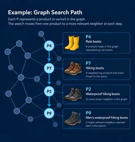
Imagine our search moving through the rain-boots graph:
If every expansion means:
visit P4 → wait for SSD visit P7 → wait for SSD visit P2 → wait for SSD visit P9 → wait for SSD
Then storage latency starts controlling search latency.
An efficient search needs to keep enough information in RAM to make good navigation decisions, while touching the SSD only when necessary. That is what makes Product Quantization important to understand.
Product Quantization: a smaller map in memory
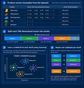
One of our product vectors stands for: “Men’s waterproof hiking boots” and may be represented as [0.12, -0.73, 0.41, 0.08, …]
The vector holds many floating-point numbers. It is not always essential to employ the full-precision vector when assessing whether a candidate merits further investigation. Product Quantization, or PQ, gives us a cheap approximation.
Before the index is searched, DiskANN trains a PQ model on representative vectors from the dataset. Training generates compact codebooks that compress dataset vectors for efficient search.
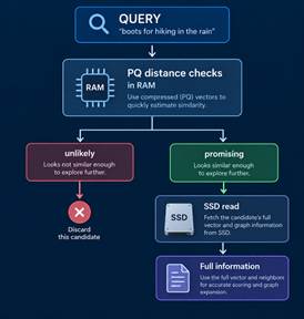
PQ trades precision for memory. The compressed vector is not identical to the original vector. Distances calculated from it are approximate. The goal of ANN Search is to identify promising candidates; not necessarily make the final ranking decision from every candidate it encounters. For our rain boots query that looks like “boots for hiking in the rain” –
PQ can help us cheaply estimate the approximate distance.
That may be enough information to decide where the graph search should go next.
PQ – ‘cheap screening stage.’
Imagine you have one billion shoes to pick from but can only have time to look at 20. You don’t need each pair’s description. You only need the 20 that are worth your time. The summary helps you screen those 20. Then you retrieve the full documents only for the shoes that matter. DiskANN uses compressed representations for the same reason.
RAM helps answer “where should I look?”
SSD holds the larger information needed when it is needed and when the graph traversal reaches the point where it is needed after the greedy-search iteration.
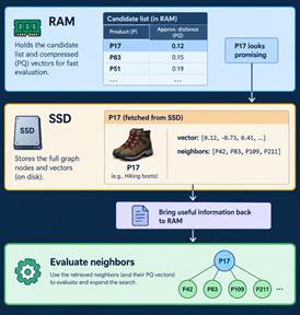
What lives on SSD?
For a graph node such as: P17 = Waterproof hiking boots The vector search cares about two things: P17, the vector, and its graph neighbors, say P42 – running boots P83 – rain boots P109 – snow boots.
When search decides that P17 is worth expanding, it needs to discover:
“What are the other nodes I can reach from P17?” It then goes to disk to reach the complete set of embeddings for P17 and gets its neighbors.
It does not read the whole index from SSD. It does selective reads driven by graph search. But SSD reads are still expensive.
The algorithm has reduced the amount of data kept in RAM. But it is still read intensive, because it still needs to fetch data for each of the neighbors, and each of that adds up to a read. The reads are sequential, which means CPU spends time waiting for storage.
DiskANN is about evaluating a list of candidates, not just one at a time.
It maintains a candidate frontier. That leads to ‘beam search’.
Beam search: give the SSD several things to do
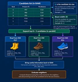
From the candidate list, instead of doing the loop of reading the node we want – wait process-read the next node, we can work several promising candidates simultaneously, as below.
That gives the storage device more parallel work and helps hide some of the latency of individual reads. The SSD-index design notes in the DiskANN repository explicitly call for beam search to explore more than one neighbor at a time and increase SSD queue depth, with asynchronous I/O used to hide waiting time.
This is why beam width becomes much more interesting once DiskANN moves to disk. Beam width depends on more than just the number of expanded candidates.
Beam width facilitates I/O parallelism by enabling simultaneous retrieval of multiple promising graph nodes, rather than performing each SSD access in a sequential manner. It may also be noteworthy that L and beam width are not the same thing.
L determines the permitted breadth of the frontier. Beam width determines the number of candidates expanded at once.
For example, L = 100 beam width = 4 does not mean we are reading 100 nodes from SSD simultaneously. It means keeping up to 100 promising candidates. From amongst them, choose a small batch of 4 to expand and search together.
On an SSD-backed index, the second knob also affects how effectively we can use the storage device. Certain graph nodes exhibit higher popularity compared to others, resulting in more frequent visits. such nodes are cached for further processing. These optimizes reads from SSD even further.
Putting the pieces together
Let’s run our rain boots query again.
“Boots for hiking in the rain”
The query is vectorized, then graph search starts in RAM.
PQ-compressed vectors speed up candidate selection, and cached graph nodes improve access efficiency.
The candidate list (L) holds the best options found so far, while beam width determines how many can be expanded at once.
Only those promising nodes require selective reading from SSD, where the larger graph and vector data live.
This lets DiskANN search for datasets far larger than RAM without reading the entire index from disk.
PQ helps make large numbers of approximate distance evaluations cheap enough to guide the search.
The graph indicates the permitted destination nodes. Takeaways are as below –
L determines how broad a set of possibilities we keep alive.
The cache prevents us from repeatedly fetching useful nodes from disk.
The SSD provides the capacity to hold an index far larger than available RAM.
Exploring only a tiny, useful portion of the vector space while still recovering the true nearest neighbors are often enough to achieve high recall.
Summary of terminologies used so far –
Term
Simple meaning
SSD index
the large graph/vector store that does not need to fit entirely in RAM
PQ
a compressed approximation of vectors used to make candidate evaluation cheaper
PQ code
the compact representation of a vector
Cache
useful graph data we keep in RAM to avoid repeated SSD reads
Cache hit
The node we need is already in RAM
Cache miss
we have to fetch the node from SSD
SSD read
fetching graph/vector information for a node we want to explore
L
how broad a candidate frontier we maintain
Beam width
how many promising candidates we expand together
I/O parallelism
having multiple SSD reads in flight instead of waiting for them one at a time
Recall
whether all these shortcuts still find the true nearest neighbors often enough
In the next and final part, we can look at how to tweak each of these knobs operationally: R, alpha, L, beam width, PQ size, memory budget, recall, latency and actually tune a DiskANN index.