The Birthday Problem – with T-SQL and R

When I was on SQLCruise recently – Buck Woody (b|t) made a interesting statement – that in a room of 23 people, there is over a 50% chance that  two or more have the same birthdays. And sure enough, we did end up having more than two people with same birthday. I was tempted to play with this rather famous problem (there is a great introductory wiki post on it here)  using statistics for a while, and got around to it this weekend. Let us test the hypothesis first.

Given a room of 23 random people, what are chances that two or more of them have the same birthday? 

This problem is a little different from the earlier ones, where we actually knew what the probability in each situation was.

What are chances that two people do NOT share the same birthday? Let us exclude leap years for now..chances that two people do not share the same birthday is 364/365, since one person’s birthday is already a given. In a group of 23 people, there are 253 possible pairs (23*22)/2. So the chances of no two people sharing a birthday is 364/365 multiplied 253 times. The chances of two people sharing a birthday, then, per basics of probability, is 1 – this. Doing the math then – first with T-SQL –

DECLARE @x INTEGER, @NUMBEROFPAIRS INTEGER, @probability_notapair numeric(18, 4), @probability_pair numeric(18, 4)
DECLARE @daysinyear numeric(18,4), @daysinyearminus1 numeric(18, 4)
SELECT @x = 23
SELECT @numberofpairs = (@x*(@x-1)/2)
SELECT @daysinyear = 365
SELECT @daysinyearminus1 = @daysinyear - 1

SELECT @probability_notapair = (@daysinyearminus1/@daysinyear)

SELECT 'Probability of a pair having birthdays' ,1-power(@probability_notapair, @NUMBEROFPAIRS)

birthday

In R this is very easily calculated using the line

prod(1-(0:22)/365)

To be aware that prod is just a function that multiplies what it is supplied, it is not a special statistical function of any kind. In this case since the math is really easy, that is all we need to calculate the result.

bday

As we can see it is pretty close to what we got with T-SQL.

We can play around with R a little bit and get a nice graph illustrating the same thing.

positiveprob <- numeric(23) #creatingvectortoholdvalues
#loop and fill values in vector
for (n in 1:23) {
 negativeprob <- 1 - (0:(n - 1))/365
 positiveprob[n] <- 1 - prod(negativeprob) }
#draw graph to show probability
plot(positiveprob, main = 'Graph of birthday probabilites for 23 people', xlab = 'Number of people in room', ylab = 'Probability of same birthdays')

bday3

As we can see the probability of two or more people sharing a birthday in a room of about 23 is near 50%. Pretty amazing.

There is a ton of very detailed posts on this rather famous problem, this is just a basic intro for those of you learning stats and R.
1 https://www.scientificamerican.com/article/bring-science-home-probability-birthday-paradox/

2 http://blog.revolutionanalytics.com/2012/06/simulating-the-birthday-problem-with-data-derived-probabilities.html

Thanks for reading!!

Normal approximation to binomial distribution using T-SQL and R

In the previous post I demonstrated the use of binomial formula to calculate probabilities of events occurring in certain situations. In this post am going to explore the same situation with a bigger sample set. Let us assume, for example, that instead of 7 smokers we had 100 smokers. We want to know what are the chances that a maximum of 35 of them have a serious lung disease. Going by the Binomial formula illustrated in the previous post that would mean a whole lot of calculations – calculating the probability of every situation less than 35 and then stick the values into the formula to derive an answer. That is a very laborious way to derive a result, even if we are using an automated process to do it.  An easier way to do it is to use the normal distribution, or central limit theorem. My post on the theorem illustrates that a sample will follow normal distribution if the sample size is large enough. We will use that as well as the rules around determining probabilities in a normal distribution, to arrive at the probability in this case.
Problem: I have a group of 100 friends who are smokers.  The probability of a random smoker having lung disease is 0.3. What are chances that a maximum of 35 people wind up with lung disease?

Step 1: How do I know my problem fits this particular statistical solution?
To determine whether n is large enough to use what statisticians call the normal approximation to the binomial, both of the following conditions must hold:

image0.png

In this case 100*0.3 = 30, which is way greater than 10. The second condition 100*0.7 is also 70 and way greater than 10. So we are good to proceed.

2 Statistically stated, we need to find P(x<=35)

3 The formula to use now is zee where ‘meu’ in the numerator is the mean and sigma, the denominator is the standard deviation. Let us use some tried and trusted t-sql to arrive at this value.

4 We use 35 as x, but we add 0.5 as suggested ‘corrective value’ to it. Running T-SQL to get z value as below:

DECLARE @X numeric(10,4), @p numeric(10, 4), @n numeric
(10, 4), @Z NUMERIC(10, 4)
DECLARE @MEAN NUMERIC(10, 4), @VARIANCE NUMERIC(10, 4), @SD NUMERIC(10, 4)
SELECT @X = 35.5
SELECT @P = 0.3
SELECT @N = 100
SELECT @MEAN = @N*@p
SELECT @VARIANCE = @N*@p*(1-@p)
SELECT @SD = SQRT(@VARIANCE)
SELECT @Z = (@X-@MEAN)/@SD
SELECT @Z as 'Z value'

zvalue

5 To calculate probability from Z value, we can use Z value tables. There are also plenty of online calculators available – I used this one.  I get probability to be 0.884969.

zvalue

6 The same calculation can be achieved with great ease in R by just saying

pbinom(35,size=100,prob=0.3)

The result I get is very close to above.

zvalue

You can get the same result by calling the R function from within TSQL as below

EXEC sp_execute_external_script
 @language = N'R'
 ,@script = N'x<-pbinom(35,size=100,prob=0.3);
 print(x);'
 ,@input_data_1 = N'SELECT 1;'

zee

In other words, there is a 88.39 percent chance that 35 out of 100 smokers end up with lung disease. Thank you for reading!


The Binomial Formula with T-SQL and R

In a previous post I explained the basics of probability. In this post I will use some of those principles to see how to solve certain problems. I will pick a very simple problem that I found in a statistics textbook. Suppose I have 7 friends who are smokers. The probability that a random smoker will develop a lung condition is 0.3. What is the probability that a maximum of 2 of them will develop a severe lung condition? To apply the binomial formula for this problem – I need the following conditions to be met:

1 The trials are independent
2 The number of trials, n is fixed.
3 Each trial outcome can be a success or a failure
4 The probability of success in each case is the same.

Applying these rules –
1 The 7 smoking friends are not related or from the same group. (This is important as one friend’s habits can influence another and that does not make for an independent trial).
2 They smoke approximately at the same rate.
3 Either they get a lung disease or they don’t. We are not considering other issues they may have because of smoking.
4 Since all these conditions are met, the probability of each of them getting a lung disease is more or less the same.

The binomial formula given that
x = total number of “successes” (pass or fail, heads or tails etc.)
P = probability of a success on an individual trial
n = number of trials
q= 1 – p – is as below:

prob

For those not math savvy the ! stands for factorial of a number. In above example n equals 7. x, The number of ‘successes’ (morbid, i know, to define a lung condition as a success but just an example) we are looking for is 2. p is given to be 0. and q is 1 – 0.3 which is 0.7.  Now, given the rules of probability – we need to add probability of 0 or none having a lung condition, 1 person having a lung condition and 2 having a lung condition – to see what is the probability of a maximum of 2 having a lung condition. Let us look at doing this with T-SQL first, then with R and then calling the R script from within T-SQL.

1 Using T-SQL:

There are a lot of different ways to write the simple code of calculating factorial. I found this one to be most handy and reused it. I created the user defined function as ‘factorial’ and used the same code below to calculate probabilities of 0.1 or 2 people getting a lung illness. If we add the 3 together we get the total probability of the maximum of 2 people getting a lung illness – which is about 0.65 or 65 %.

DECLARE @n decimal(10,2), @x decimal(10, 2), @p decimal(10, 2), @q decimal(10, 2)
DECLARE @p0 decimal(10, 2), @p1 decimal(10, 2), @p2 decimal(10, 2), @n1 decimal(10, 2), @n2 decimal(10, 2), @n3 decimal(10, 2)
SELECT @n = 7, @x = 0, @p = 0.3,@q=0.7
SELECT @x = 0
SELECT @n1 = dbo.factorial(@n) 
SELECT @n2 = dbo.factorial(@n-@x)
SELECT @n3 = 1

SELECT @p1 = ( @n1/(@n2 * @n3))*power(@p, @x)*power(@q,@n-@x)
select @p1 as 'Probability of 0 people getting lung illness'

SELECT @x = 1
SELECT @p1 = ( @n/@x)*power(@p, @x)*power(@q,@n-@x)
select @p1 as 'Probability of 1 person getting lung illness'

SELECT @x = 2
SELECT @n1 = dbo.factorial(@n) 
SELECT @n2 = dbo.factorial(@n-@x)
SELECT @n3 = dbo.factorial(@x)
SELECT @p2 = ( @n1/(@n2 * @n3))*power(@p, @x)*power(@q,@n-@x)
select @p2 as 'Probability of 2 people getting lung illness'


Results are as below:

prob1

2 Using R:

The R function for this is seriously simple, one line call as below.

dbinom(0:2, size=7, prob=0.3)

My results, almost exactly the same as what we got with T-SQL.

prob2

3 Calling R from T-SQL:

Instead of writing all that code i can simply call this function from with TSQL –

EXEC sp_execute_external_script
 @language = N'R'
 ,@script = N'x<-dbinom(0:2, size=7, prob=0.3);
 print(x);'
 ,@input_data_1 = N'SELECT 1;'

Results as below:

prob3

It is a LOT of fun to get our numbers to tie in more than one way. Thanks for reading.


Sampling Distribution and Central Limit Theorem

In this post am going to explain (in highly simplified terms) two very important statistical concepts – the sampling distribution and central limit  theorem.

The sampling distribution is the distribution of means collected from random samples taken from a population. So, for example, if i have a population of life expectancies around the globe. I draw five different samples from it. For each sample set I calculate the mean. The collection of those means would make up my sample distribution. Generally, the mean of the sample distribution will equal the mean of the population, and the standard deviation of the sample distribution will equal the standard deviation of the population.

The central limit theorem states that the sampling distribution of the mean of any independent,random variable will be normal or nearly normal, if the sample size is large enough. How large is “large enough”? The answer depends on two factors.

  • Requirements for accuracy. The more closely the sampling distribution needs to resemble a normal distribution, the more sample points will be required.
  • The shape of the underlying population. The more closely the original population resembles a normal distribution, the fewer sample points will be required. (from stattrek.com).

The main use of the sampling distribution is to verify the accuracy of many statistics and population they were based upon.

Let me try demonstrating this with an example in TSQL. I am going to use [Production].[WorkOrder] table from Adventureworks2016. To begin with, am going to test if this data is actually a normal distribution in of itself. I use the Empirical rule test I have described here for this.  Running the code for the test, I get values that tell me that this data is very skewed and hence not a normal distribution.

DECLARE @sdev numeric(18,2), @mean numeric(18, 2), @sigma1 numeric(18, 2), @sigma2 numeric(18, 2), @sigma3 numeric(18, 2)
DECLARE @totalcount numeric(18, 2)
SELECT @sdev = SQRT(var(orderqty)) FROM [Production].[WorkOrder]
SELECT @mean = sum(orderqty)/count(*) FROM [Production].[WorkOrder]
SELECT @totalcount = count(*) FROM [Production].[WorkOrder] where orderqty > 0

SELECT @sigma1 = (count(*)/@totalcount)*100 FROM [Production].[WorkOrder] WHERE orderqty >= @mean-@sdev and orderqty<= @mean+@sdev
SELECT @sigma2 = (count(*)/@totalcount)*100 FROM [Production].[WorkOrder] WHERE orderqty >= @mean-(2*@sdev) and orderqty<= @mean+(2*@sdev)
SELECT @sigma3 = (count(*)/@totalcount)*100 FROM [Production].[WorkOrder] WHERE orderqty >= @mean-(3*@sdev) and orderqty<= @mean+(3*@sdev)

SELECT @sigma1 AS 'Percentage in one SD FROM mean', @sigma2 AS 'Percentage in two SD FROM mean', @sigma3 as 'Percentage in 3 SD FROM mean

In order for the data to be a normal distribution – the following conditions have to be met –

68% of data falls within the first standard deviation from the mean.
95% fall within two standard deviations.
99.7% fall within three standard deviations.

The results we get from above query suggest to us that the raw data does not quite align with these rules and hence is not a normal distribution.

pic1

Now, let us create a sampling distribution from this. To do this we need to pull a few random samples of the data. I used the query suggested here to pull random samples from tables. I pull 30 samples in all and put them into tables.

 SELECT * INTO [Production].[WorkOrderSample20]
 FROM [Production].[WorkOrder]
 WHERE (ABS(CAST((BINARY_CHECKSUM(*) * RAND()) as int)) % 100) < 20

I run this query 30 times and change the name of the table the results go into, so am now left with 30 tables with random samples of data from main table.

Now, I have to calculate the mean of each sample, pool it all together and then re run the test for normal distribution to see what we get. I do all of that below.

DECLARE @samplingdist TABLE (samplemean INT)
 
 INSERT INTO @samplingdist (samplemean)
 select sum(orderqty)/count(*) from [Production].[WorkOrderSample1]

 INSERT INTO @samplingdist (samplemean)
 select sum(orderqty)/count(*) from [Production].[WorkOrderSample2]
 
 INSERT INTO @samplingdist (samplemean)
 select sum(orderqty)/count(*) from [Production].[WorkOrderSample3]
 
 INSERT INTO @samplingdist (samplemean)
 select sum(orderqty)/count(*) from [Production].[WorkOrderSample4]

 INSERT INTO @samplingdist (samplemean)
 select sum(orderqty)/count(*) from [Production].[WorkOrderSample5]

 INSERT INTO @samplingdist (samplemean)
 select sum(orderqty)/count(*) from [Production].[WorkOrderSample6]

 INSERT INTO @samplingdist (samplemean)
 select sum(orderqty)/count(*) from [Production].[WorkOrderSample7]

 INSERT INTO @samplingdist (samplemean)
 select sum(orderqty)/count(*) from [Production].[WorkOrderSample8]

 INSERT INTO @samplingdist (samplemean)
 select sum(orderqty)/count(*) from [Production].[WorkOrderSample9]

 INSERT INTO @samplingdist (samplemean)
 select sum(orderqty)/count(*) from [Production].[WorkOrderSample10]

 INSERT INTO @samplingdist (samplemean)
 select sum(orderqty)/count(*) from [Production].[WorkOrderSample11]

 INSERT INTO @samplingdist (samplemean)
 select sum(orderqty)/count(*) from [Production].[WorkOrderSample12]

 INSERT INTO @samplingdist (samplemean)
 select sum(orderqty)/count(*) from [Production].[WorkOrderSample13]

 INSERT INTO @samplingdist (samplemean)
 select sum(orderqty)/count(*) from [Production].[WorkOrderSample14]

 INSERT INTO @samplingdist (samplemean)
 select sum(orderqty)/count(*) from [Production].[WorkOrderSample15]

 INSERT INTO @samplingdist (samplemean)
 select sum(orderqty)/count(*) from [Production].[WorkOrderSample16]

 INSERT INTO @samplingdist (samplemean)
 select sum(orderqty)/count(*) from [Production].[WorkOrderSample17]

 INSERT INTO @samplingdist (samplemean)
 select sum(orderqty)/count(*) from [Production].[WorkOrderSample18]

 INSERT INTO @samplingdist (samplemean)
 select sum(orderqty)/count(*) from [Production].[WorkOrderSample19]

 INSERT INTO @samplingdist (samplemean)
 select sum(orderqty)/count(*) from [Production].[WorkOrderSample20]

 INSERT INTO @samplingdist (samplemean)
 select sum(orderqty)/count(*) from [Production].[WorkOrderSample21]

 INSERT INTO @samplingdist (samplemean)
 select sum(orderqty)/count(*) from [Production].[WorkOrderSample22]

 INSERT INTO @samplingdist (samplemean)
 select sum(orderqty)/count(*) from [Production].[WorkOrderSample23]

 INSERT INTO @samplingdist (samplemean)
 select sum(orderqty)/count(*) from [Production].[WorkOrderSample24]

 INSERT INTO @samplingdist (samplemean)
 select sum(orderqty)/count(*) from [Production].[WorkOrderSample25]

 INSERT INTO @samplingdist (samplemean)
 select sum(orderqty)/count(*) from [Production].[WorkOrderSample26]

 INSERT INTO @samplingdist (samplemean)
 select sum(orderqty)/count(*) from [Production].[WorkOrderSample27]

 INSERT INTO @samplingdist (samplemean)
 select sum(orderqty)/count(*) from [Production].[WorkOrderSample28]

 INSERT INTO @samplingdist (samplemean)
 select sum(orderqty)/count(*) from [Production].[WorkOrderSample29]

 INSERT INTO @samplingdist (samplemean)
 select sum(orderqty)/count(*) from [Production].[WorkOrderSample30]


DECLARE @sdev numeric(18,2), @mean numeric(18, 2), @sigma1 numeric(18, 2), @sigma2 numeric(18, 2), @sigma3 numeric(18, 2)
DECLARE @totalcount numeric(18, 2)
SELECT @sdev = SQRT(var(samplemean)) FROM @samplingdist
SELECT @mean = sum(samplemean)/count(*) FROM @samplingdist
SELECT @totalcount = count(*) FROM @samplingdist
SELECT @sigma1 = (count(*)/@totalcount)*100 FROM @samplingdist WHERE samplemean >= @mean-@sdev and samplemean<= @mean+@sdev
SELECT @sigma2 = (count(*)/@totalcount)*100 FROM @samplingdist WHERE samplemean >= @mean-(2*@sdev) and samplemean<= @mean+(2*@sdev)
SELECT @sigma3 = (count(*)/@totalcount)*100 FROM @samplingdist WHERE samplemean >= @mean-(3*@sdev) and samplemean<= @mean+(3*@sdev)

SELECT @sigma1 AS 'Percentage in one SD FROM mean', @sigma2 AS 'Percentage in two SD FROM mean', 
@sigma3 as 'Percentage in 3 SD FROM mean'The results I get are as below.

pic2

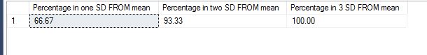
The results seem to be close to what is needed for a normal distribution now.

(68% of data should fall within the first standard deviation from the mean.
95% should fall within two standard deviations.
99.7% should fall within three standard deviations.)

It is almost magical how easily the rule fits. To get this to work  I had to work on many different sampling sizes – to remember the rule says that it needs considerable number of samples to reflect a normal distribution. In the next post I will look into some examples of using R for demonstrating the same theorem. Thank you for reading.
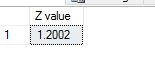
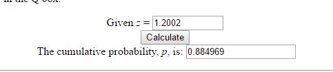