Descriptive Statistics with SQL and R – II

In the previous post I looked into some very basic and common measures of descriptive statistics – mean, median and mode, and how to derive these using T-SQL, R as well as a combo of the two in SQL Server 2016. These measures also called measures of ‘Central Tendency‘. In this post am going to describe some measures called ‘Measures of Dispersion‘. Dispersion refers to how much the said value differs from the average and how many such values are distributed around the average.

Below are 4 very common measures of dispersion –

  1. Range
  2. Inter-Quartile Range
  3. Variance
  4. Standard Deviation

The first and most common measure of dispersion is called ‘Range‘. The range is just the difference between the maximum and minimum values in the dataset. It tells you how much gap there is between the two and therefore how wide the dataset is in terms of its values. It is however, quite misleading when you have outliers in the data. If you have one value that is very large or very small that can skew the Range and does not really mean you have values spanning the minimum to the maximum.

To lower this kind of an issue with outliers – a second variation of the range called Inter-Quartile Range, or IQR is used. The IQR is calculated by dividing the dataset into 4 equal parts after sorting the said value in ascending order. For the first and third part, the maximum values are taken and then subtracted from each other. The IQR ensures that you are looking at top and near-bottom ranges and therefore the value it gives is probably spanning the range.

A more accurate calculation of dispersion is called Variance. Variance is the average of the difference between each value and the mean, divided by the number of values. When your dataset is comprised of an entire population the number of values are the total number of values, but when it is comprised of a sample, the number of values are deducted by 1 to ensure a statistical adjustment. The larger the variance, the more widespread the values are.

The last measure of dispersion am going to look into in this post is Standard Deviation.The Standard Deviation is the square root of the variance. The smaller the standard deviation, the lesser is the dispersion around the mean. The larger, the greater.

The higher the values of variance and standard deviation – the more skewed your data is and the less likely it is to lend itself to any real statistical analysis or even forecasting or predictive reporting.

I used the same data set that I did in the earlier post to run queries for this. Details on that can be found here.

Using T-SQL:

Below are my T-SQL queries to derive range, inter quartile range, variance and standard deviation. I was surprised to find that T-SQL actually has a built in function for variance, which makes it very easy. Was not sure why this particular function would exist when the vast majority of other statistical functions don’t, but makes sense to use it since it does 🙂

–Calculate range of the dataset
SELECT MAX(AGE) – MIN(AGE) as Range FROM [dbo].[WHO_LifeExpectancy]

–Calculate Interquartile range of the dataset
SELECT MAX(QUARTILEMAX) – MIN(QUARTILEMAX) AS INTERQUARTILERANGE
FROM
(SELECT QUARTILE, MAX(AGE) AS QUARTILEMAX FROM (SELECT NTILE(4) OVER ( ORDER BY Age ) AS Quartile ,
Age FROM [dbo].[WHO_LifeExpectancy]) A
GROUP BY QUARTILE HAVING QUARTILE = 1 OR QUARTILE = 3) A

–Calculate variance of the datasest
SELECT VAR(Age) AS VARIANCE FROM [dbo].[WHO_LifeExpectancy]

–Calculate standard deviation of the dataset
SELECT SQRT(VAR(Age)) AS STDDEV FROM [dbo].[WHO_LifeExpectancy]

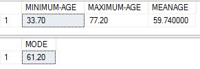
Results are as below:

descstats2

Using R:

The R script to do the exact same thing is as below. None of these calculations require anything more than calling a packaged function in R, which is why it is usually the preferred way to do it.

#load necessary libraries and connect to the database
install.packages(“RODBC”)
library(RODBC)

cn <- odbcDriverConnect(connection=”Driver={SQL Server Native Client 11.0};server=MALATH-PC\\SQL01;database=WorldHealth;Uid=sa;Pwd=<password>”)
data <- sqlQuery(cn, ‘select age from [dbo].[WHO_LifeExpectancy] where age is not null’)

#Get range
agerange <- max(data)-min(data)
agerange

#Get Interquartile Range
interquartileagerange <- IQR(unlist(data))
interquartileagerange

#Get Variance
variance <- var(data)
variance

#Get Standard Deviation
stddev <- sd(unlist(data))
stddev

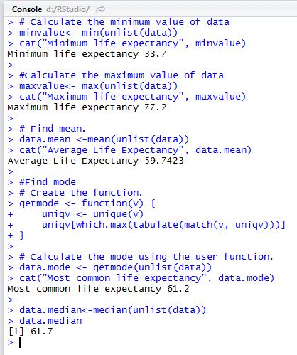
The results you get, almost exact matches to what T-SQL gave us:

descstats2-R

3. Using R function calls with T-SQL

Now the last part , where we call the R script via T-SQL. We have to make small changes to the script – the ‘cat’ function to concatenate results, /n to introduce a carriage return for readability and removing the ‘unlist’ that native R needs because of how R structures data it reads directly from SQL . But for this the math is exactly the same.

 — calculate  simple dispersion measures
EXEC sp_execute_external_script
@language = N’R’
,@script = N’ range <-max(InputDataSet$LifeExpectancies)-min(InputDataSet$LifeExpectancies)
cat(“Range”, range,”\n”);
InterquartileRange <-IQR(InputDataSet$LifeExpectancies)
cat(“InterQuartileRange”, InterquartileRange,”\n”);
variance <-var(InputDataSet$LifeExpectancies)
cat(“Variance”, variance,”\n”);
stdeviation <-sd(InputDataSet$LifeExpectancies)
cat(“StdDeviation”, stdeviation,”\n”);’
,@input_data_1 = N’SELECT LifeExpectancies = Age FROM [WorldHealth].[dbo].[WHO_LifeExpectancy];’
;

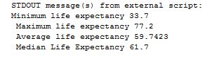
And the results, exactly the same as the two above:

descstats2-sqlandr

It has been fun so far doing this in 3 different ways and getting the same results. But as we go into more advanced statistics it will not be that simple. It will, however, definitely help us understand how far we can push statistical math with T-SQL, how easy and simple it is with R, and what can/cannot be done in the first version of calling R from within T-SQL. I can’t wait to play with it further and blog as I go along.

Thank you for reading.


Descriptive Statistics with SQL and R – 1

I started my re-discovery of statistics with an introduction here. This second post is about descriptive statistics – very basic, simple statistics you begin with as a learner. Descriptive Statistics are also called Summary Statistics and serve to describe/summarize the data. They allow you to understand what the data is about and get a feel for its common features. There are two types of descriptive statistics

  1. Measures of Central Tendency – for example, mean, median and mode.
  2. Measures of Dispersion – or variation from Central Tendency such as standard deviation, interquartile range and so on.

You can figure out minimum and maximum values, outliers, average and most frequently occuring values with descriptive statistics. It takes you no further than that – it is not for deeper diagnostics of data, predictive or prescriptive analytics – but it is where you begin with in terms of understanding your data. In this post I took 5 very basic measures of descriptive statistics in category 1 for my specific measure – which is life expectancy across the globe.

  1. Minimum life expectancy
  2. Maximum life expectancy
  3. Mean or Average life expectancy
  4. Median or Central/mid point value of life expectancy
  5. Mode or most common life expectancy.

It is easy to understand what are minimum and maximum values.They help you understand how wide the data set is. Some people also look at number of nulls in the dataset.
Mean or average is the sum of all values divided by number of values. Mean is very commonly used but does a poor job when there are outliers in the data such an unsually large or small value that can skew the average value.
Median is what you see as mid-point on a sorted scale of values. In other words median is the physical center of the data.Since median is not mathematically based it is rarely used in calculations. It does help with outliers better than mean does.
Mode is the most common value – very useful when you need to know to understand what are the values that occur most frequently. Mode can be used on nominal and ordinal data, hence it is the most commonly used measure of central tendency. There can be more than one mode in a sample.

The formulas to derive at these values are relatively simple – I tried them using both T-SQL and R, and also calling the R script via SQL. T-SQL is not really the best tool for statistical analysis, although it is useful for a beginner to get started.R are on the other hand has built-in functions for most of this.

With R integration into SQL Server 2016 we can pull an R script and integrate it rather easily. I will be covering all 3 approaches. I am using a small dataset – a single table with 915 rows, with a SQL Server 2016 installation and R Studio. The complexities of doing this type of analysis in the real world with bigger datasets involve setting various options for performance and dealing with memory issues – because R is very memory intensive and single threaded.

My table and the data it contains can be created with scripts here. For this specific post I used just one column in the table – age. For further posts I will be using the other fields such as country and gender.

Using T-SQL:

Below are my T-SQL Queries to get minimum, maximum, mean and mode.  The mode is rather difficult using T-SQL. Given how easy it is do with R, I did not spend a lot of time on it. How to arrive at the mode of a dataset using T-SQL has been researched well and information can be found here for those interested.

SELECT MIN(age) AS [MINIMUM-AGE],MAX(age) AS [MAXIMUM-AGE],
ROUND((SUM(age)/COUNT(*)),2) AS MEANAGE FROM [dbo].[WHO_LifeExpectancy]
WHERE AGE IS NOT NULL

SELECT TOP 1 AGE AS MODE FROM [dbo].[WHO_LifeExpectancy]
GROUP BY AGE
ORDER BY count(*) DESC

The results I got were as below:
sql-results

Using R:

I downloaded and installed R Studio from here. The script should work just the same with any other version of R.
Before running the actual functions to get results, one has to load up the right libraries in R and connect to the database, then load the table contents into what is called a dataframe in R.Below commands help us do that.

install.packages(“RODBC”)
library(RODBC)

cn <- odbcDriverConnect(connection=”Driver={SQL Server Native Client 11.0};server=MALATH-PC\\SQL;database=WorldHealth;Uid=sa;Pwd=<password>”)

data <- sqlQuery(cn, ‘select age from [dbo].[WHO_LifeExpectancy] where age is not null’)

The data in my table is now in a dataframe called ‘data’ with R. To run statistical functions I need to ‘unpivot’ the dataframe into a single vector, and I have to use the ‘unlist‘ function in R for that purpose. When I run the R script via SQL, this is not necessary as it reads directly from the SQL tables. The R script i used to get the values is as below.

# Calculate the minimum value of data
minvalue<- min(unlist(data))
cat(“Minimum life expectancy”, minvalue)

#Calculate the maximum value of data
maxvalue<-max(unlist(data))
cat(“Maximum life expectancy”, maxvalue)

# Find mean.
data.mean <-mean(unlist(data))
cat(“Average Life Expectancy”, data.mean)

#Find mode
# Create the function.
getmode <- function(v) {
uniqv <- unique(v)
uniqv[which.max(tabulate(match(v, uniqv)))]
}

# Calculate the mode using the user function.
data.mode <- getmode(unlist(data))
cat(“Most common life expectancy”, data.mode)

data.median<-median(unlist(data))
data.median

Note that aside from mode all the rest are built-in functions in R. I borrowed the code for mode from here (the cool thing about R is the huge # of pre written scripts to do just about anything).

The results  I got are as below:

r-studio

To be noted that the values of max, min, mean and mode are exactly the same as what we got from T-SQL which means this is correct.

3. Using R function calls with T-SQL

Details on configuration needed to use R within SQL Server are explained here.

The last and final step was to try the same script, without certain R specific commans such as ‘unlist’ to unlist the dataframe, and ‘cat’ to display concatenated results.  The scripts are as below. The first one is the call to basic statistics and the second is to get the mode. I separated the function for mode into a script in itself as it was multiple lines and hard to include within same call.

EXEC sp_execute_external_script
@language = N’R’
,@script = N’minvalue <-min(InputDataSet$LifeExpectancies);
cat(“Minimum life expectancy”, minvalue,”\n”);
maxvalue <-max(InputDataSet$LifeExpectancies);
cat(” Maximum life expectancy”, maxvalue,”\n”);
average <-mean(InputDataSet$LifeExpectancies);
cat(” Average life expectancy”, average,”\n”);
medianle <-median(InputDataSet$LifeExpectancies);
cat(” Median Life Expectancy”, medianle,”\n”);

,@input_data_1 = N’SELECT LifeExpectancies = Age FROM [WorldHealth].[dbo].[WHO_LifeExpectancy];’
;

EXEC sp_execute_external_script
@language = N’R’
,@script = N’getmode <- function(v) {
uniqv <- unique(v)
uniqv[which.max(tabulate(match(v, uniqv)))]
};
modele <- getmode(InputDataSet$LifeExpectancies);
cat(” Most Common Life Expectancy”, modele);

,@input_data_1 = N’SELECT LifeExpectancies = Age FROM [WorldHealth].[dbo].[WHO_LifeExpectancy];’
;

sql-r-results

Other than a slight variation in mode , which i suspect is because of decimal rounding issues, the results are exactly the same as what we got via TSQL and R Studio.

In the next post I am going to deal with measure of dispersion. Thank you for reading and do leave me comments if you can!


Basic Statistics with SQL – Introduction

I was a student of statistics in school and college. I didn’t get to use much of anything I learned at school, and this was considered one of them. But apparently with the boom in interest in data mining, knowledge of statistics has become more important than ever before. Along with learning basics of statistics comes numerous tools available to mine data, and get appropriate metrics for business. For many people including me – we’d like to get involved with meaningful data mining but don’t know where to start. I personally decided to go back into revising some concepts I knew back in the days off the top of my head. I am going to blog every week on one concept that I am re-learning and applying to some data. I have great interest in data related to healthcare, so I used a data set available for public download from World Health Organization to help me. I also used T-SQL to run basic statistical queries. T-SQL is far from the best tool there is for statistical analysis, but it is certainly useful for getting a start on the subject of understanding and summarizing data.

You are given a dataset. It could a table, or multiple tables. What are the appropriate questions to ask before you get around to analyzing/mining this dataset? Below are a few that are recommended that I found useful to begin with:

  1. What is the variable being measured? (There may be multiple, but for simplicity’s sake, let us make it 1).
    In my case that is life expectancy of people around the globe,summarized at country level.
  2. What is the population used? (The population is the potential collection of people that are ideally part of the sample used.)
    People living in the countries around the globe.
  3. What is the sample used? (The sample is the subset of the population used for this specific purpose)
    People living in the countries targeted for this study.

The reason for asking these questions is to ensure that the dataset is representative of what we intend to present – if we say we are presenting statistics on global life expectancy there better be numbers related to that from many different countries around the world. There need not be every country on the list, but several countries are necessary to make the sample worthy of study. Sampling and sample size is in itself a very vast and deep subject. But this is just about understanding its basics and why we ask certain questions.

The last question that would determine the nature of our queries is about type of the variable being measured. Data used for statistical analysis can fall into one of 4 categories ,also called statistical scales – Nominal, Ordinal, Interval and Ratio. Like it is with rules of normalization – there are 4 rules to determine nature of measurement –

  1. Identity  – each value is unique
  2. Magnitude – values have a relationship to each other
  3. Equal Intervals – difference between two unique values is the same
  4. Minimum value of 0 – the minimal value of the variable is 0.

Applying these rules to the above types of data –

Nominal data is what falls into specific mutually exclusive categories (the ones commonly under radio buttons) – male/female, ethnicity, nationality and so on. It satisfies rule 1.

Ordinal data is basically nominal data but has buckets that are gradeable or have some sort of order to them – such as ‘how good was this presentation – excellent to horrible’, or ‘how do you feel’, or even for example, work related titles – like data entry clerk, programmer, dba, senior dba and so on. It satisfies rules 1 and 2.

Interval data is numbers,  and like ordinal – very specific numbers but you can calculate the difference between them.  Interval data satisfies rules 1,2 and 3 but not 4 – because it does not stop at 0. An example would be temperature.

Ratio data is numbers like interval data but the minimum stops at 0. This enables data to be ratio friendly and hence is the best kind for statistical analysis.Examples would be weight, speed of a vehicle and so on.

In my specific data set – the variable am analyzing is life expectancies/age, which is ratio data by some and ordinal by others. This link addresses why.  (There are a lot of such ambiguities and in the end what we call it is secondary to the value we derive out it).  Now that i know my data, i need to go about running some basic statistics on it. More on that in the next post.